Chapter 4
This is an article that was given to me by my math prof at NDSU and was apparently printed in Skyscraper Engineer (vol. 25, no. 2) and then reprinted in Minnesota Technology, Spring of 1985. It has been reprinted here with permission of the author. Copyright is owned by the author, Joe Samosky. The illustrations were created by David King. Please do not reprint or copy this article in part or in its entirety without first obtaining permission from the author.
(For those of you who are thinking you've seen this before, I had put it up and found out shortly thereafter that I was in violation of copyright, so I then took it down. I was able to track down the author, who very kindly granted me permission, which is why I'm putting it back up now.)
Chapter Four
By Joe Samosky
You know the story. It's several weeks into the term and you've finally reached it: Chapter Four. It seems that every textbook in the sciences and engineering has a Chapter Four, although it isn't always the fourth chapter of the book. Usually, however, it goes something like this...
4.1 Introduction
Up until now, in our development of statistical quantum anthropomorphism we have relied on a rather intuitive mathematical background underlying the examples presented in chapters two and three. The authors assume that the student has had no previous experience with quantum anthropomorphic vector space transformations, except for an introductory course in multivariate vector calculus of complex hyperbolic spheroids, taken in the freshman or sophomore years.
4.2 Notational Conventions
A complete explanation of the symbolic notation used in the following development may be found in "Gersplatzen Fumblebach uben Vierdenthalen und Ischengargen," J. Steinman et. al., Annalen der Physike, Vol. 3, No. 2 (1874). The authors have made minor modifications to this system. These changes are discussed in Appendix K of the supplementary text Quantum Anthropomorphism - A Simple Approach. The conventions are not rigid, however, and students are encouraged to fabricate their own symbols at will, as we will frequently do.
4.3 Derivation of Antoliodore's Equation
We begin with the equation of poikilothermic electrostatics, the experimental derviation of which is found in Chapter 11:

(1)
Rearranging, we obtain

(2)
We now multiply both sides of equation (2) by the permittivity of free space, eo:

(3)
Through simple algebraic manipulation we obtain
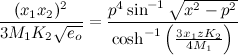
(4)
The intermediate steps above are left as an exercise for the reader (Problem 4.4a).
We now state as fact the following equation, the proof of which is beyond the scope of this text1:

(5)
Squaring both sides,

(6)
and multiplying by the permittivity of free space, eo:

(7)
Finally, we multiply and divide equation (7) by Avogadro's number (NA = 6.023•1023) and raise both sides to the power numerically equal to the price per pound of bananas (expressed in drachmas) in Helsinki, Finland on July 23, 1972. (This last quantity, Svordenbjorg's constant, is an empirically derived value discussed more fully in the preface to the supplementary text Basic Statistical Quantum Anthropomorphism for the Life and Social Sciences - Second Edition.)
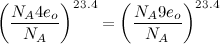
(8)
Substituting the above into equation (4) we obtain the desired relation, Antoliodore's equation, which will lead directly to the proof of the McWorthstead-Landellier Theorem.

(9)
where C=M1/K2.
Expressed in words, equation (9) states that x is directly dependent on p. That is, if p increases in value, x also increases. It is also true that if p decreases in value, x will decrease. Finally, it can be shown from (9) that if p remains constant, so will x. The reader should convince himself or herself of the above assertions before proceeding.
4.4 Proof of the McWorthstead-Landellier Theorem
With these concepts now mastered, we can proceed with our proof of what is the most fundamental principle of statistical quantum anthropomorphism, the McWorthstead-Landellier Theorem (MLT). A formal mathematical statement of the MLT is rather abstract, and beyond the scope of this introductory discussion. In simple terms, the theorem asserts that if, in a suitable rectangularly tesselated region of n-dimensional anthropomorphic vector space, a counter current mass flow function satisfies boundary conditions so as to ensure compliance with the Cauchy-Schwartz inequality for any chosen combination of state-transition subsets, then the closed line integral in n-space around a loop of Henle (starting at a singularity point and proceeding clockwise) will be indentically equal to zero. In other words, if a counter current mass flow function satisfies the Cauchy-Schwartz inequality compatible boundary conditions (for any chosen combination of state-transition subsets) in an appropriate rectangularly tesselated region of anthropomorphic vector n-space, then the closed n-space line integral from a singularity point clockwise around a loop of Henle will equal zero, identically. Intuitively, this implies that the entropy of the universe increases for any spontaneous process. (The proof of this is left as a supplementary exercise for the reader.)
We shall only demonstrate the proof of the MLT for 3-space; the extrapolation to higher dimensional spaces should be obvious. Figure 1(a) shows the standard i-x-p convention for our three coordinate axes. Note that each axis is at an angle of 90 degrees (a right angle) to each of the other two. They are said to be orthogonal (from the Greek orthogonios: ortho - straight, right, true; gonia - angle. Similar to the Gothic gawrisqan - to bring fruit, or the Sanskrit urdhva - upright or high, and vardhate - he increases.) Note also that the rotation from axis i to axis x gives axis p by the right-hand rule: the coordinate system is said to be right-handed. We use dotted lines to show the negative portions of the axes, solid lines to show the positive regions. Finally, note that the i axis is directed upward, the p axis is directed to the right and the x axis is directed out of the plane of the page.

Next we graph Antoliodore's Equation (9) in Figure 1(b)2. C has been chosen as an arbitrary positive constant. The reader should observe the direct dependence of x upon p, as was previous described. Note that the slope of the line (defined as rise/run) is equal to C, and that the line passes through the origin at point O (where (x,i,p) = (0,0,0)).
If the reader has been attentive and has closely followed the discussion to this point, the remaining steps in teh proof should be clear. Omitting the intermediate algebra, we illustrate the result in Figure 1(c)3. The singularity points are indicated at A and B, with the loop of Henle designated by I. Clearly, the closed clockwise line integral around the loop will equal zero (identically), thus establishing our proof (Q.E.D.).
4.5 Conclusion
In this chapter we have formalized some of the concepts introduced in the first section of the text. Antoliodore's Equation was developed and utilized in our proof of the important McWorthstead-Landellier Theorem. Our approach was largely intuitive and nonmathematical, in order to provide the student with an appreciation of the simplicity and beauty of quantum anthropomorphic principles. Readers desiring a more rigorous foundation in the material presented are reffered to Chapter Four of the supplementary text Statistical Quantum Anthropomorphism: What More Can Be Said? (Second Edition).
[1] For a complete proof see "Applications of the Uncertainly Principle to Applied Arithmetic," B. Mugglesdorf, Journal of Applied Mathematics, Vol. 56, No. 9 (1969).
[2] The i and x axes have been interchanged and the positive and negative regions of the graph have been switched in the illustration for the sake of clarity.
[3] Note that we have rotated the principle axes and redesigned the original x-i-p axes as s-r-j so as to avoid confusion.
(For those of you who are thinking you've seen this before, I had put it up and found out shortly thereafter that I was in violation of copyright, so I then took it down. I was able to track down the author, who very kindly granted me permission, which is why I'm putting it back up now.)
Chapter Four
By Joe Samosky
You know the story. It's several weeks into the term and you've finally reached it: Chapter Four. It seems that every textbook in the sciences and engineering has a Chapter Four, although it isn't always the fourth chapter of the book. Usually, however, it goes something like this...
4.1 Introduction
Up until now, in our development of statistical quantum anthropomorphism we have relied on a rather intuitive mathematical background underlying the examples presented in chapters two and three. The authors assume that the student has had no previous experience with quantum anthropomorphic vector space transformations, except for an introductory course in multivariate vector calculus of complex hyperbolic spheroids, taken in the freshman or sophomore years.
4.2 Notational Conventions
A complete explanation of the symbolic notation used in the following development may be found in "Gersplatzen Fumblebach uben Vierdenthalen und Ischengargen," J. Steinman et. al., Annalen der Physike, Vol. 3, No. 2 (1874). The authors have made minor modifications to this system. These changes are discussed in Appendix K of the supplementary text Quantum Anthropomorphism - A Simple Approach. The conventions are not rigid, however, and students are encouraged to fabricate their own symbols at will, as we will frequently do.
4.3 Derivation of Antoliodore's Equation
We begin with the equation of poikilothermic electrostatics, the experimental derviation of which is found in Chapter 11:
(1)
Rearranging, we obtain
(2)
We now multiply both sides of equation (2) by the permittivity of free space, eo:
(3)
Through simple algebraic manipulation we obtain
(4)
The intermediate steps above are left as an exercise for the reader (Problem 4.4a).
We now state as fact the following equation, the proof of which is beyond the scope of this text1:
(5)
Squaring both sides,
(6)
and multiplying by the permittivity of free space, eo:
(7)
Finally, we multiply and divide equation (7) by Avogadro's number (NA = 6.023•1023) and raise both sides to the power numerically equal to the price per pound of bananas (expressed in drachmas) in Helsinki, Finland on July 23, 1972. (This last quantity, Svordenbjorg's constant, is an empirically derived value discussed more fully in the preface to the supplementary text Basic Statistical Quantum Anthropomorphism for the Life and Social Sciences - Second Edition.)
(8)
Substituting the above into equation (4) we obtain the desired relation, Antoliodore's equation, which will lead directly to the proof of the McWorthstead-Landellier Theorem.
(9)
where C=M1/K2.
Expressed in words, equation (9) states that x is directly dependent on p. That is, if p increases in value, x also increases. It is also true that if p decreases in value, x will decrease. Finally, it can be shown from (9) that if p remains constant, so will x. The reader should convince himself or herself of the above assertions before proceeding.
4.4 Proof of the McWorthstead-Landellier Theorem
With these concepts now mastered, we can proceed with our proof of what is the most fundamental principle of statistical quantum anthropomorphism, the McWorthstead-Landellier Theorem (MLT). A formal mathematical statement of the MLT is rather abstract, and beyond the scope of this introductory discussion. In simple terms, the theorem asserts that if, in a suitable rectangularly tesselated region of n-dimensional anthropomorphic vector space, a counter current mass flow function satisfies boundary conditions so as to ensure compliance with the Cauchy-Schwartz inequality for any chosen combination of state-transition subsets, then the closed line integral in n-space around a loop of Henle (starting at a singularity point and proceeding clockwise) will be indentically equal to zero. In other words, if a counter current mass flow function satisfies the Cauchy-Schwartz inequality compatible boundary conditions (for any chosen combination of state-transition subsets) in an appropriate rectangularly tesselated region of anthropomorphic vector n-space, then the closed n-space line integral from a singularity point clockwise around a loop of Henle will equal zero, identically. Intuitively, this implies that the entropy of the universe increases for any spontaneous process. (The proof of this is left as a supplementary exercise for the reader.)
We shall only demonstrate the proof of the MLT for 3-space; the extrapolation to higher dimensional spaces should be obvious. Figure 1(a) shows the standard i-x-p convention for our three coordinate axes. Note that each axis is at an angle of 90 degrees (a right angle) to each of the other two. They are said to be orthogonal (from the Greek orthogonios: ortho - straight, right, true; gonia - angle. Similar to the Gothic gawrisqan - to bring fruit, or the Sanskrit urdhva - upright or high, and vardhate - he increases.) Note also that the rotation from axis i to axis x gives axis p by the right-hand rule: the coordinate system is said to be right-handed. We use dotted lines to show the negative portions of the axes, solid lines to show the positive regions. Finally, note that the i axis is directed upward, the p axis is directed to the right and the x axis is directed out of the plane of the page.
Next we graph Antoliodore's Equation (9) in Figure 1(b)2. C has been chosen as an arbitrary positive constant. The reader should observe the direct dependence of x upon p, as was previous described. Note that the slope of the line (defined as rise/run) is equal to C, and that the line passes through the origin at point O (where (x,i,p) = (0,0,0)).
If the reader has been attentive and has closely followed the discussion to this point, the remaining steps in teh proof should be clear. Omitting the intermediate algebra, we illustrate the result in Figure 1(c)3. The singularity points are indicated at A and B, with the loop of Henle designated by I. Clearly, the closed clockwise line integral around the loop will equal zero (identically), thus establishing our proof (Q.E.D.).
4.5 Conclusion
In this chapter we have formalized some of the concepts introduced in the first section of the text. Antoliodore's Equation was developed and utilized in our proof of the important McWorthstead-Landellier Theorem. Our approach was largely intuitive and nonmathematical, in order to provide the student with an appreciation of the simplicity and beauty of quantum anthropomorphic principles. Readers desiring a more rigorous foundation in the material presented are reffered to Chapter Four of the supplementary text Statistical Quantum Anthropomorphism: What More Can Be Said? (Second Edition).
[1] For a complete proof see "Applications of the Uncertainly Principle to Applied Arithmetic," B. Mugglesdorf, Journal of Applied Mathematics, Vol. 56, No. 9 (1969).
[2] The i and x axes have been interchanged and the positive and negative regions of the graph have been switched in the illustration for the sake of clarity.
[3] Note that we have rotated the principle axes and redesigned the original x-i-p axes as s-r-j so as to avoid confusion.